V.  MODELING, SIMILARITY, AND DIMENSIONAL ANALYSIS

To this point, we have concentrated on analytical methods of solution for fluids problems.

 

However, analytical methods are not always satisfactory due to:
(1)   limitations due to simplifications required in the analysis,
(2)   complexity and/or expense of a detailed analysis.

The most common alternative is to:
Use experimental test & verification procedures.

However, without planning and organization, experimental procedures can :

(a)   be time consuming,
(b)   lack direction,
(c)   be expensive.

This is particularly true when the test program necessitates testing at one set of conditions, geometry, and fluid with the objective to represent a different but similar set of conditions, geometry, and fluid.

 

Dimensional analysis provides a procedure that will typically reduce both the time and expense of experimental work necessary to experimentally represent a desired set of conditions and geometry.

 

It also provides a means of "normalizing" the final results for a range of test conditions.   A normalized (non-dimensional) set of results for one test condition can be used to predict the performance at different but dynamically similar conditions (including even a different fluid).

 

The basic procedure for dimensional analysis can be summarized as follows:

1.  Compile a list of relevant variables (dependent & independent) for the problem being considered,
2.  Use an appropriate procedure to identify both the number and form of the resulting non-dimensional parameters.

Buckingham Pi Theorem
The procedure most commonly used to identify both the number and form of the appropriate non-dimensional parameters is referred to as the Buckingham Pi Theorem.  The theorem uses the following definitions:

n  =  the number of independent variables relevant to the problem
j’  =  the number of independent dimensions found in the n variables
j   =  the reduction possible in the number of variables necessary to be considered simultaneously
k  =  the number of independent P terms that can be identified to describe the problem,  k  =  n - j

Summary of Steps:

1. List and count the n variables involved in the problem.
2. List the dimensions of each variable using {MLTQ} or {FLTQ}.  Count the number of basic dimensions (j’) for the list of variables being considered.
3. Find j by initially assuming j  =  j’ and look for j repeating variables which do not form a pi product.  If not successful, reduce j by 1 and repeat the process.
4. Select j scaling, repeating variables which do not form a P product.
5. Form a P term by adding one additional variable and form a power product.  Algebraically find the values of the exponents which make the product dimensionless.  Repeat the process with each of the remaining variables.
6. Write the combination of dimensionless pi terms in functional form:

Pk  =  f( P1, P2, …Pi)
P  Theorem Example
Consider the following example for viscous pipe flow.  The relevant variables for this problem are summarized as follows:

DP = pressure drop       r = density           V =  velocity      D = diameter
m = viscosity                  e = roughness       L = length
Seven  pipe flow variables:        {DP            r,  V,  D,  m,  e,  L }

                                                 dependent                independent

Use of the Buckingham Pi Theorem proceeds as follows:

1.   Number of independent variables:   n  = 7

2.   List the dimensions of each variable  ( use  m L t Q ):

variables        DP        r         V        D          m         e       L
dimensions  mL-1t-2      mL-3         Lt-1        L            mL-1t-1        L          L

 

The number of basic dimensions is  j’ = 3 (m, L, t).

3.   Choose   j =  3 with the repeating variables being   r,  V,  and  D.  They do not form a dimensionless P term.  No combination of the 3 variables will eliminate the mass dimension in density or the time dimension in velocity.  

4.   This step is described in step 3.  The repeating variables again are r,  V,  and  D and j = 3.  Therefore,  k =  n – j = 7 – 3  =  4 independent P terms.

5.   Form the P   terms:

      P1  =  ra Vb Dc m-1 =  (mL-3)a ( Lt-1)b Lc ( mL-1t-1 )-1

In order for the P term to have no net dimensions, the sum of the exponents for each dimension must be zero.  Therefore, summing the exponents for each dimension, we have:

mass:          a  -  1  = 0 ,   a =  1
time:           - b  +  1  =  0,    b  = 1
length:         -3a  + b  +  c + 1  =  0,  c =  3 – 1 – 1  =  1

We therefore have

                   P1  =  r V D /m  =   Re =  Reynolds number

Note: Changing the initial exponent for m to 1 ( from -1) would result in the reciprocal of the same non-dimensional groups.  Thus, some experience is useful in obtaining P terms consistent with existing theory.

Repeating the process with the roughness,  e
P2 =  ra Vb Dc e1 =  (mL-3)a ( Lt-1)b Lc ( L )1

Solving:

mass:          a    = 0 ,   a =  0
time:           - b  =  0,    b  = 0
Length:       -3a  + b  +  c + 1  =  0,  c =  – 1

P2 =  e / D                  Roughness ratio

Repeat the process with the length  L.

P3 =  ra Vb Dc L1 =  (mL-3)a ( Lt-1)b Lc ( L )1

Solving:

mass:          a    = 0 ,   a =  0
time:           - b  =  0,    b  = 0
length:         -3a  + b  +  c + 1  =  0,  c =  – 1

P3 =  L / D                  length-to-diameter ratio

These three are the independent  P  terms.

Now obtain the dependent P term by adding  DP

P4 =  ra Vb Dc DP1 =  (mL-3)a ( Lt-1)b Lc ( mL-1t-2 )1

Solving:

mass:          a  +  1  = 0 ,   a =  -1
time:           - b  - 2 =  0,    b  = -2
length:         -3a  + b  +  c - 1  =  0,  c =  0

P4 =  DP / r V2           Pressure coefficient

Application of the Buckingham Pi Theorem to the previous list of variables yields the following non-dimensional combinations:

or

 

Thus, a non-dimensional pressure loss coefficient for viscous pipe flow would be expected to be a function of (1) the Reynolds number, (2) a non-dimensional pipe length, and (3) a non-dimensional pipe roughness.  This will be shown to be exactly the case in Ch. VI, Viscous Internal Flow.

A list of typical dimensionless groups important in fluid mechanics is given in the accompanying table.

    From these results, we would now use a planned experiment with data analysis techniques to get the exact form of the relationship among these non - dimensional parameters.

The next major step is concerned with the design and organization of the experimental test program.

Two key elements in the test program are:
*   design of the model
*   specification of the test conditions, particularly when the test must be performed at conditions similar to, but not the same as the conditions of interest.

Similarity and Non-dimensional Scaling

 

The basic requirement in this process is to achieve 'similarity' between the 'experimental model and its test conditions' and the 'prototype and its test conditions' in the experiment. 

Table 5.2  Dimensional Analysis and Similarity

Parameter	Definition	Qualitative ratio of effects	Importance
Reynolds number			Always
Mach number			Compressible flow
Froude number			Free-surface flow
Weber number			Free-surface flow
Cavitation number (Euler number)			Cavitation
Prandtl number			Heat convection
Eckert number			Dissipation
Specific-heat ratio			Compressible flow
Strouhal number			Oscillating flow
Roughness ratio			Turbulent,rough walls
Grashof number			Natural convection
Temperature ratio			Heat transfer
Pressure coefficient			Aerodynamics, hydrodynamics
Lift coefficient			Aerodynamics hydrodynamics
Drag coefficient			Aerodynamics, hydrodynamics

In this context, “similarity” is defined as

 

Similarity:  All relevant dimensionless parameters have the same values for the model and the prototype.

Similarity generally includes three basic classifications in fluid mechanics:

(1)  Geometric similarity
(2)  Kinematic similarity
(3)  Dynamic similarity

 

Geometric similarity

 

In fluid mechanics, geometric similarity is defined as follows:

 

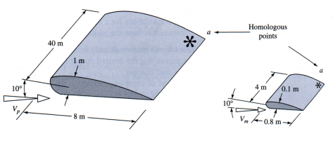
Geometric Similarity:   All linear dimensions of the model are related to the corresponding dimensions of the prototype by a constant scale factor SFG .     

Consider the following airfoil section (Fig. 5.4):

Fig. 5.4  Geometric Similarity in Model Testing

For this case, geometric similarity requires the following:

In addition, in geometric similarity:

All angles are preserved.
All flow directions are preserved.
Orientation with respect to the surroundings must be same for the model and the prototype, i.e.

Angle of attack )m = angle of attack )p

Kinematic Similarity

In fluid mechanics, kinematic similarity is defined as follows:

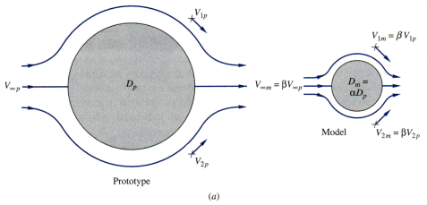
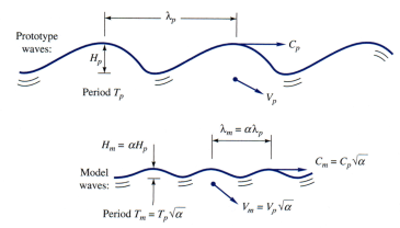
Kinematic Similarity:   The velocities at 'corresponding' points on the model & prototype are in the same direction and differ by a constant scale factor   SFk.

Therefore, the flows must have similar streamline patterns.

Flow regimes must be the same.

These conditions are demonstrated for two flow conditions, as shown in the following kinematically similar flows (Fig. 5.6).

Fig. 5.6a  Kinematically Similar Low Speed Flows

Fig. 5.6b Kinematically Similar Free Surface Flows

The conditions of kinematic similarity are generally met automatically when geometric and dynamic similarity conditions are satisfied.

 

Dynamic Similarity

In fluid mechanics, dynamic similarity is typically defined as follows:

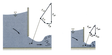
Dynamic Similarity:      This is basically met if model and prototype forces differ by a constant scale factor at similar points.

This is illustrated in the following figure for flow through a sluice gate (Fig. 5.7).

Fig. 5.7  Dynamic Similarity for Flow through a Sluice Gate

This is generally met for the following conditions:

1.  Compressible flows:      model & prototype   Re, Ma,   are equal

Rem  =  Rep,    Mam=  Map  ,    gm  =  gp

 

2. Incompressible flows

     a.  no free surface

                  Rem  =  Rep

     b.  flow with a free surface

                  Rem  =  Rep      ,  Frm  =  Frp

 

Note:  The parameters being considered, e.g. velocity, density, viscosity, diameter, length, etc.,  generally relate to the flow, geometry, and fluid characteristics of the problem and are considered to be independent variables for the subject problem.

 

The result of achieving similarity by the above means is that relevant non - dimensional dependent variables, e.g. CD, Cp, Cf, or Nu, etc., are then equal for both the model and prototype. 

This result would then indicate how the relevant dependent results, e.g. drag force, pressure forces, viscous forces, are to be scaled for the model to the prototype. 

Equality of the relevant non-dimensional independent variables, Re, Ma, x/L, etc.,  indicates how the various independent variables of importance should be scaled.

An example of this scaling is shown as follows:

 

The drag on a sonar transducer prototype is to be predicted based on the following wind tunnel model data and prototype data requirements.   Determine the model test velocity  Vm   necessary to achieve similarity and the expected prototype force  Fp   based on the model wind tunnel test results.

Given:	Prototype	Model
	sphere	sphere
D	1 ft	6 in
V	5 knots	unknown?
F	?	5.58 lbf
r	1.98	0.00238
n	1.4 *10-5	1.56 * 10-4

 

From dimensional analysis:

 

For the prototype, the actual operating velocity and Reynolds number are

 

Prototype:            

 

Equality of Reynolds number then yields the required model test velocity of

Based on actual test results for the model, i.e. measured Fm, equality of model and prototype drag coefficients yields

Note:  All fluid dynamic flows and resulting flow characteristics are not Re dependent.

Example:

The drag coefficient for bluff bodies with a fixed point of separation; e.g. radar antennae,  generally have a constant, fixed number for CD which is not a function of Re.