Differential equations of fluid motion

IV.  DIFFERENTIAL RELATIONS FOR A FLUID PARTICLE

This chapter presents the development and application of the basic differential equations of fluid motion.  Simplifications in the general equations and common boundary conditions are presented that allow exact solutions to be obtained.  Two of the most common simplifications are 1) steady flow and 2) incompressible flow.

The Acceleration Field of a Fluid

A general expression of the flow field velocity vector is given by

One of two reference frames can be used to specify the flow field characteristics

eulerian – the coordinates are fixed and we observe the flow field
characteristics as it passes by the fixed coordinates.

lagrangian  - the coordinates move through the flow field following individual
particles in the flow.

Since the primary equation used in specifying the flow field velocity is based on Newton’s second law, the acceleration vector is an important solution parameter.  In cartesian coordinates, this is expressed as

total    local                   convective

The acceleration vector is expressed in terms of three types of derivatives:

    Total acceleration =  total derivative of velocity vector

     = local derivative  +  convective derivative  of velocity vector

Likewise, the total derivative (also referred to as the substantial derivative ) of other variables can be expressed in a similar form, e.g.

Example 4.1

Given the eulerian velocity-vector field

find the acceleration of the particle.

For the given velocity vector, the individual components are

                   u  =  3 t                 v =  x z                  w  =  t y2

Evaluating the individual components for the acceleration vector, we obtain

           =  3 i  +  0 j  +  y2 k

            =  z j               =  2 t y k                =  x j

Substituting, we obtain

  =  ( 3 i  +  y2 k)  +  (3 t) (z j)  +  (x z) (2 t y k)  +  (t y2) (x j)

After collecting terms, we have

  =  3 i + (3 t z + t x y2) j + ( 2 x y z t + y2) k    ans.

The Differential Equation of Conservation of Mass

If we apply the basic concepts of conservation of mass to a differential control volume, we obtain a differential form for the continuity equation in cartesian coordinates:

in cylindrical coordinates:

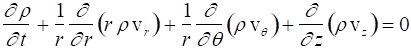
and in vector form:

                                     

Steady Compressible Flow

For steady flow, the term   =  0  and all properties are function of position only.

The previous equations simplify to

Cartesian: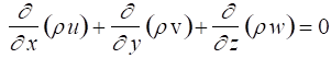            

Cylindrical: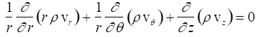         

Incompressible Flow

For incompressible flow, density changes are negligible, r = const., and     =  0

In the two coordinate systems, we have
Cartesian:            
Cylindrical:         

Key Point:

It is noted that the assumption of incompressible flow is not restricted to fluids which cannot be compressed, e.g. liquids.  Incompressible flow is valid for
(1) when the fluid is essentially incompressible (liquids) and (2) for compressible fluids for which compressibility effects are not significant for the problem being considered.

The second case is assumed to be met when the Mach number is less than 0.3:

                   Ma = V/c  < 0.3     For these conditions, gas flows can be considered                             incompressible

 

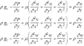
The Differential Equation of Linear Momentum

If we apply Newton’s Second Law of Motion to a differential control volume we obtain the three components of the differential equation of linear momentum.  In cartesian coordinates, the equations are expressed in the form:

 

Inviscid Flow:  Euler’s Equation

If we assume the flow is frictionless, all of the shear stress terms drop out. The resulting equation is known as Euler’s equation and in vector form is given by

where    is the total or substantial derivative of the velocity  as discussed previously and    is the usual vector gradient of pressure.  This form of Euler’s equation can be integrated along a streamline to obtain the frictionless Bernoulli’s equation ( Sec. 4.9). 

 

Newtonian Fluid:  Constant Density and Viscosity

For Newtonian fluids, viscous stresses are proportional to fluid element strain rates and the coefficient of viscosity, m.  For incompressible flow with constant density and viscosity, the Navier Stokes equations become

Review example 4.5 in the text.

Differential Equation of Angular Momentum

Application of the integral angular-momentum equation to a differential element and taking moments about the z,y, and x axes respectively yields the interesting result

or

Thus, the shear stresses are symmetric and there is no differential form of the angular momentum equation.

The Differential Equation of Energy

The differential equation of energy is obtained by applying the first law of thermodynamics to a differential control volume.  The most complex element of the development is the differential form of the control volume work due to both normal and tangential viscous forces.  When this is done, the resulting equation has the form

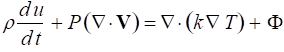
where  is the viscous dissipation function and accounts for the frictional conversion of fluid energy into heat.  The term for the total derivative of internal energy includes both the transient and convective terms seen previously.

Two common assumptions used to simplify the general equation are

                   1.   du ≈ Cv dT     and  2.  Cv, m, k, r  ≈ constants

With these assumptions, the energy equation reduces to

It is noted that the flow-work term was eliminated as a result of the assumption of constant density, r, for which the continuity equation becomes    ,thus eliminating the term  .

For the special case of a fluid at rest with constant properties, the energy equation simplifies to the familiar heat conduction equation,

We now have the three basic differential equations necessary to obtain complete flow field solutions of fluid flow problems.

Boundary Conditions for the Basic Equations

In vector form, the three basic governing equations are written as

Continuity: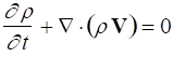          

Momentum: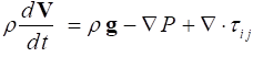         

Energy:                

We have three equations and five unknowns:  r, V, P, u, and T ;  and thus need two additional equations.  These would be the equations of state describing the variation of density and internal energy as functions of P and T, i.e.

                                      r =   r (P,T)  and  u = u (P,T)

Two common assumptions providing this information are either:

1. Ideal gas:                    r =  P/RT   and    du =  Cv dT

2. Incompressible fluid:   r = constant   and  du  =  C dT

Time and Spatial Boundary Conditions

Time Boundary Conditions:  If the flow is unsteady, the variation of each of the variables (r, V, P, u, and T ) must be specified initially, t = 0, as functions of spatial coordinates, e.g. x,y,z.

Spatial Boundary Conditions:  The most common spatial boundary conditions are those specified at a fluid – surface boundary.  This typically takes the form of assuming equilibrium (e.g. no slip condition – no property jump) between the fluid and the surface at the boundary.

This takes the form:

                                      Vfluid  =  Vwall     Tfluid  =  Twall

Note that for porous surfaces with mass injection, the wall velocity will be equal to the injection velocity at the surface.

A second common spatial boundary condition is to specify the values of  V, P, and T at any flow inlet or exit.

Example 4.6

For steady incompressible laminar flow through a long tube, the velocity distribution is given by

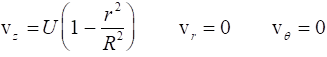
where U is the maximum or centerline velocity and R is the tube radius.  If the wall temperature is constant at Tw and the temperature  T  =  T(r) only, find T(r) for this flow.

For the given conditions, the energy equation reduces to

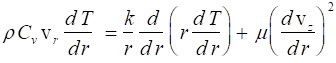
Substituting for vz and realizing the vr = 0, we obtain

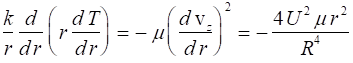
Multiply by r/k and integrate to obtain

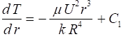
Integrate a second time to obtain

Since the term, ln r, approaches infinity as r approaches 0, C1 = 0.

Applying the wall boundary condition, T = Tw at r = R, we obtain for C2

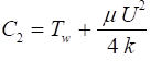
The final solution then becomes

 

The Stream Function

The necessity to obtain solutions for multiple variables in multiple governing equations presents an obvious mathematical challenge.  However, the stream function, Y, allows the continuity equation to be eliminated and the momentum equation solved directly for the single variable, Y.  The use of the stream function works for cases when the continuity equation can be reduced to only two terms. 

For example, for 2-D, incompressible flow, continuity becomes

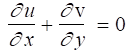
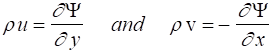
Defining the velocity components to be

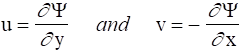
which when substituted into the continuity equation yields

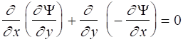
and continuity is automatically satisfied.

 

Geometric interpretation of Y

It is easily shown that lines of constant   Y  are flow streamlines.  Since flow does not cross a streamline, for any two points in the flow we can write

Thus the volume flow rate between two points in the flow is equal to the difference in the stream function between the two points.

 

Steady Plane Compressible Flow

In like manner, for steady, 2-D, compressible flow, the continuity equation is

For this problem, the stream function can be defined such that

As before, lines of constant stream function are streamlines for the flow, but the change in stream function is now related to the local mass flow rate by

 

Vorticity and Irrotationality

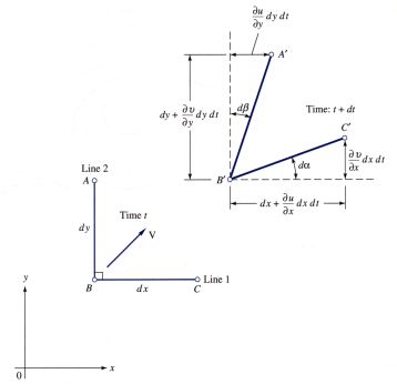
The concepts of vorticity and irrotationality are very useful in analyzing many fluid problems.  The analysis starts with the concept of angular velocity in a flow field.

Consider three points, A, B, & C, initially perpendicular at time t, that then move and deform to have the position and orientation at t + dt.  The lines AB and BC have both changed length and incurred angular rotation da and db relative to their initial positions.

Fig. 4.10 Angular velocity and strain rate of two fluid lines deforming in the x-y plane

We define the angular velocity wz about the z axis as the average rate of counter-clockwise turning of the two lines expressed as

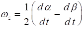
Applying the geometric properties of the deformation shown in Fig. 4.10 and taking the limit as Dt  ® 0, we obtain

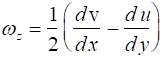
In like manner, the angular velocities about the remaining two axes are

                                

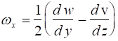
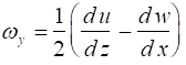
From vector calculus, the angular velocity can be expressed as a vector with the form

          w  =  i w x  +  j w y  +  k wz  = 1/2 the curl of the velocity vector, e.g.

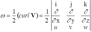
The factor of  2  is eliminated by defining the vorticity, x  ,  as follows:

x = 2 w  = curl V

 

Frictionless Irrotational Flows

When a flow is both frictionless and irrotational, the momentum equation reduces to Euler’s equation given previously by

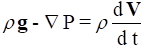
As shown in the text, this can be integrated along the path, ds, of a streamline through the flow to obtain

For steady, incompressible flow this reduces to

constant along a streamline

which is Bernoulli’s equation for steady incompressible flow as developed in Ch. III.

Velocity Potential

The condition of irrotationalty allows the development of a scalar function, f, similar to the stream function as follows:

                   If                         then           

where  f  =  f(x,y,z,t) and is called the velocity potential function.  The individual velocity components are obtained from  f  with

Orthogonality

For irrotational and 2-D flow, both Y and f exist and the streamlines and potential lines are perpendicular throughout the flow regime.  Thus for incompressible flow in the x-y plane we have

                                             and            

and both relations satisfy Laplace’s equation.

Review example 4.9 in the text.

Examples of Plane Potential Flow

The following section shows several examples of the use of the stream function and velocity potential to describe specific flow situations, in particular three plane potential flows.  These flows are shown graphically in Fig. 4.12.

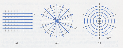
Fig. 4.12  Three plane potential flows

 

Uniform Stream in the x Direction
For a uniform velocity flow represented by  V  =  U i , both a velocity potential and stream function can be defined. The flow field is shown in Fig. 4.12a and f and Y are found as follows:

                           and                

Integrating these expressions and setting the constants of integration equal to zero we obtain

                                            and                

Line Source or Sink at the Origin
In potential flow, a source is a point in a flow field which provides a point source of flow.  For the case where the z-axis is treated as a line source with fluid supplied uniformly along its length, a stream function and velocity potential can be defined in 2-D polar coordinates starting with

                               

Integrating and discarding the constants of integration as before, we obtain the equations for  Y  and  f  for a simple, radial flow, line source, or sink:

Y = m q       and      f = m ln r
The flow field is shown schematically in Fig. 4.12b for a uniform source flow.

Line Irrotational Vortex
A 2-D line vortex is a purely circulating, steady motion with vq = f(r) only and vr = 0.  This flow is shown schematically in Fig. 4.12c.  For irrotational flow, this is referred to as a free vortex and the stream function and velocity potential function may be found from

                           and            

where K is a constant.  Again, integrating, we obtain for Y  and  f

Y = - K ln r       and      f = K q

The strength of the vortex is defined by the constant K.

Review additional examples for combinations of uniform flow, a source, and a sink in the text.