First: A Recap of First Order Circuits
We know how to find the response, x(t), of any first order circuit. 
(And by response, we mean a current or a voltage,
usually an inductor current or a capacitor voltage.)

The response will always look like this:

where

• The first term (Ae– t/t ) is the natural response or called the transient part of the solution
• The second term (e–t/t ò y(t) e t/t dt) is the forced response or called the steady state solution.
•  t  is called the time constant       =  RC             -or-     = L/R
• y(t) is called the forcing function =  vs(t) / t       -or-      = is(t) / t
• A is an arbitrary constant evaluated from the initial condition of the  circuit,
  i.e. either the initial capacitor voltage or the initial inductor current.

For the special case of a constant forcing function the response looks like this:

These results came from our previous work. 
In case you forgot, this is how we did it:

• First, we obtainted the Thevenin or Norton equivalent circuit from the perspective of the energy storage element (the inductor or the capacitor).
• Next we found the first order differential equation that describes the circuit:

where x, t and y(t) are defined above

• Then we solved this first order differential equation:  x(t)  = xn(t) + xf(t).
• To find the transient part of the response, set y(t) = 0 and solve the equation. 
  Note that, in general, the natural response of a differential equation will have as many arbitrary constants as the order of the equation.
  
• To find the forced part of the response, the original differential equation is solved by guessing a response that has the same form as the forcing function.

Now: Second Order Circuits
i.e. circuits with two (irreducible) energy storage elements
These circuits are described by a second order differential equation. 
Hence they are called second order circuits. 

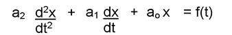
The most general form of a 2nd order differential equation is:  

The solution to these will be a bit more complex than for first order circuits.

The steps to solving higher order circuits:

• Find the differential equation (d.e.) that describes the circuit.
• Solve the d.e. by finding the complete solution, x(t):
• First find the natural response, xn(t).
  (It will have the same number of arbitrary constants as the order of the d.e.
  Beware! It is tempting to find the value of the constants at this stage. DON’T!)
• Then find the forced response, xf(t).
• Finally, put them together to get the complete response:  x(t) = xn + xf
• After you have the complete response, find the arbitrary constants in the solution.

 
Step 1:  Finding the differential equation of a circuit
Use the State Variable Method. (Steps are on the next page.)
This method can be extended to circuits with any number of energy storage elements.

Step 2a:  Finding the natural response
The natural response, xn(t), is found by setting the forcing function of the differential equation to zero. The natural response will have the same number of arbitrary constants as the order of the differential equation. (Don’t try to solve for these constants yet.) Usually this response will die out as t gets large. So it is also called the transient response. 

Step 2b:  Finding the forced response
The forced response, xf(t), must satisfy the differential equation with no arbitrary constants.  Find it by guessing a solution that is the most general form as the forcing function and substitute it into the differential equation to determine the constants.

Step 2c:  Finding the complete response
Put them together:  x = xn + xf

Step 3:  Finding the arbitrary constants in the solution
Once you have the complete response, use the initial conditions of the circuit to solve for the arbitrary constants. 
Beware:  Don’t try to solve for these constants until you have both the natural response and the forced response.  You need to use the complete response to plug the initial conditions into, not just the natural response.

The above gives the big picture.  Now we will delve into the details.

State Variable Method
for finding differential equation of a nth order circuit

First find the nth order differential equation for the circuit:

1. Identify a set of n state variables.
   Note:
   There are many possible sets.
   The best choice is usually all of the capacitor voltages and all of the inductor currents.
   So for a 3rd order circuit with 2 capacitors and 1 inductor the set might look like this: v1, v2, i1
2. Obtain n equations in n unknowns.
   Note:
   The equations will all be 1st order differential equations.
   The unknowns will be the state variables identified in step #1.
   (So if you get a variable in one of the equations and it is not a state variable, then you need to change it so that it is!)
   The easiest way to do this step is to use NVA or MCA.
3. Transform the n equations you just got in the previous step using s operator.
   This will give n algebraic equations in terms of s and the n unknown state variables.
4. Solve for the unknowns using Cramer’s Rule
   Rewrite the n equations of the previous step in a column so that the state variables are lined up and their coefficients are clearly shown in front of them. Everything else should be on the other side of the equation.
   It will look something like this:
   (a11) v1  +  (a12) v2  +  (a13) i1 = y1(t)
   (a21) v1  +  (a22) v2  +  (a23) i1 = y2(t)
   (a31) v1  +  (a32) v2  +  (a33) i1 = y2(t)
   Now use Cramer's rule to solve for any state variable you desire to find.
   For instance:
   .
   
5. Rearrange the equation of step #4 so that Q(s) v2 =P(s) and then convert the s operator back to derivatives.
   

This is the second-order differential equation for the circuit!

Now find the natural response:

6. Obtain the characteristic equation of the circuit by setting the determinant of Cramer's rule equal to zero.
7. Determine the roots of the characteristic equation. 
8. From the roots of the characteristic equation determine the form of the natural response. 
   (For a second order circuit there are only three possibilities.)

Now find the forced response:

9. Determine the forced response xf(t) by guessing a solution, xg(t).
   This guess should be the most general form of the forcing function.
   (For example if the forcing function, xf(t) = 3t2, then your guess should be xg(t) = K2t2 + K1t + K0)
   Substitute the guess into the differential equation and determine the constants (K0, K1, K2 …) in it.
   

Now find the complete response:

10. The complete solution: x(t) = xn(t) + xf(t)
    (This will have the arbitrary constants A1 , A2 ….An that came from the natural response)

Now find the arbitrary constants:

11. Determine the boundary conditions for the state variables. 
    (For example you can determine the initial conditions for the n state variables and use those.
    These will be the initial capacitor voltages and initial inductor currents.)
12. Find the arbitrary constants A1 , A2 ….An from the boundary conditions.
1. Plug in the b.c. into each of the first-order differential equations found in Step #2.
   This will allow you to obtain values for dx(0)/dt ….dnx(0)/dtn .
2. Using x(t) = xn(t) + xf(t), find dx(0)/dt ….dnx(0)/dtn. 
   Equate these to the values obtained in a.

Finding the natural response, xn(t), of a second order circuit
For the differntial equation:

We guess a solution of:                             xn(t) = Aest
Substitute this guess into the differential equation and simplify:    a2s2 + a1s + ao = 0
This is called the characteristic equation of the differential equation. 
It is also known as the characteristic equation of the circuit.  
Solve for the roots, s1 and s2, of the characteristic equation:
The natural response is thus:   xn(t)= A1es1t  +  A2es2t    
We are happy with this answer since we need a solution that has as many arbitrary constants as the degree of the equation. However, there are 3 possible cases for the values of the roots, s1 and s2, and these different values will alter the character of the natural response.
The roots of the characteristic equation determine the character of the natural response.

Case 1:  The Overdamped Response
The roots are negative, real and distinct: (a1/2a2)2  > (a0/ a2)
There is no problem here.
The solution is simply what we determined above.

Case 2:  The Critically Damped Response
The roots are negative, real and indistinct:  (a1/2a2)2  = (a0/ a2)
Here we have a problem.  xn(t) = (A1 + A2)est = A3est  is a solution with only one arbitrary constant.
This is not OK!  (Because this is a second order circuit we know we need 2!)
So we need to go back and guess a different solution to the differential equation. 
Let’s try xn (t) = (A1 +  A2t) est. 
After substituting this into the differential equation, with some work, we find that it works.
So for this case the solution is:

Case 3:  The Underdamped Response
The roots are distinct and complex:  (a1/2a2)2  < (a0/ a2)
There is no problem here. Complex numbers don’t scare us.
The solution is simply what we determined above.
However, we can manipulate this solution with Euler’s theorem:  cos q + j sinq = ejq
and after a bit of algebraic work this solution will be in a preferred form:

The Source Free Parallel RLC Circuit

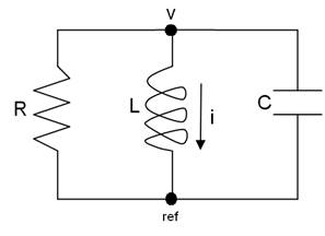
L & C may have initial energy storage:                                                      
iL(0) = Io  
                                                           vC(0) = Vo                                                                                   

The second order differential equation for this circuit is:

The natural solution is will depend on the roots of the characteristic equation.

These roots, s1 and s2, will depend on the values of R, L and C.

There are 3 possibilies for the values of the roots which correspond to the 3 cases for the natural response of the circuit:

• Overdamped
• Critically Damped
• Underdamped

To make the solution of this equation more manageable, we define the following:
Let:
a   =  1 /(2RC)                     = neper frequency or exponential damping coefficient
wo  =  1 /(LC)1/2                    = resonant (radian) frequency
wd  =  (wo2 – a2)1/2                = damped resonant frequency
j   =  a/wo                                         = damping ratio (dimensionless)
(Note that all except the damping ratio have units of sec-1.)
Hence the roots are:

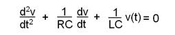
The curves shown here start at 0 which means that the initial voltage across the capacitor was 0.

Overdamped Response: a > wo 
s1, s2  are negative, real and distinct: LC > 4R2C2

                                                                                                                                    
Critically Damped Response: a = wo
s1, s2  are negative, real and same: LC = 4R2C2              


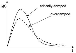
Underdamped Response: a < wo
s1, s2  are distinct and complex:  LC < 4R2C2)

Notes:                                                                                                                                            

• A1 and A2 are arbitrary constants which are determined by the initial conditions.
• The response becomes oscillatory when underdamping is present.
• tm is the time at which the maximum value is reached.
• ts, the settling time, is the time at which the value is 1% of the maximum.
• The minimum settling time occurs for slight underdamping.
• For the same values of L and C, a larger R gives a smaller maximum response. (i.e. more damping.)
• An increase in R from an overdamped system to get critical damping gives a shorter settling time.

The Source Free Series RLC Circuit

L & C may have initial energy storage:                                  
iL(0) = Io                                                       
vC(0) = Vo                                                                                    

The second order differential equation for this circuit is:
            
Depending on the values of R, L and C, the natural response will be either
Overdamped, Critically Damped or Underdamped.

As with the parallel circuit, to make the solution of this more manageable, we define the following:
Let:
                        a   =  R/(2L)                          = neper frequency or exponential damping coefficient
wo  =  1/ (LC)1/2                     = resonant (radian) frequency
wd  =  (wo2 – a2)1/2                = natural resonant frequency
j   =  a/wo                                      = damping ratio (dimensionless)
Note: the first is the only one that is different from the parallel RLC circuit.
Hence:
s1, s2 = – a + (a2 – wo2)1/2   = complex frequencies or natural frequencies

Overdamped Response:  a > wo                                                  
s1, s2  are negative, real and distinct: LC > 4L2/R2

                                                                                                                                             

Critically Damped Response:  a = wo
s1, s2  are negative, real and equal: LC = 4L2/R2

Underdamped Response: a < wo
s1, s2  are distinct and complex:  LC < 4R2C2   

                                                              
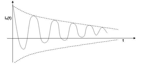
Note:
Although this is the dual of the underdamped case for the parallel RLC circuit, it looks different because this particular solution has less damping. Hence the oscillatory nature of the response is more evident. Also, the initial current was not zero here.

Finding the Forced Response, xf(t) of a Second Order Circuit

The forced response must satisfy the differential equation with no arbitrary constants. 

To find it, just guess a form for the forced response that is the most general form of the forcing function:

The constants of the assumed solutions (A, B and C) are determined by substituting the assumed solution back into the differential equation.

Note:
If one of the natural response terms has the same form as the forcing function then we need another form of the forced response.
In general we can use xf = tP xn1 where the integer P is selected so that xf is not duplicated in natural response. (Use the lowest value).
In these cases the forced solution will not have exactly the same form as the forcing function.