Trained teams

Several roles have been defined in the Six Sigma strategy:

• Champions: business leaders, provide resources and support implementation
• Master Black Belts: experts and culture-changers, train and mentor Black Belts/Green Belts
• Black Belts: lead Six Sigma project teams
• Green Belts: carry out Six Sigma projects related to their jobs

Sigma levels

2σ: logic and intuition are enough, no special tool is required
3-4σ: quality programs used by US companies for years (seven tools)
5σ: DMAIC, process characterization and optimization
6σ: DFSS (DMADOV), design for Six Sigma

Focusing of the Xs

X are the inputs of the process, Y the output
Traditionally, companies focused on the Y, Six Sigma forces us to understand the relationship between the Xs and Y to find the vital Xs and control them.

The five phases

Define - Customer expectations of the process?
Measure - What is the frequency of defects?
Analyze - Why, when and where do defects occur?
Improve - How can we fix the process?
Control - How can we make the process stay fixed?

DFSS

Design
1 Identify product/process performance and reliability CTQs and set quality goals
Measure
2 Perform CTQ flowdown to subsystems and components
3 Measurement system analysis/capability
Analyze
4 Develop conceptual designs (benchmarking, tradeoff analysis)
5 Statistical analysis of any relevant data to assess capability of conceptual designs
6 Build scorecard with initial product/process performance and reliability estimates
7 Develop risk assessment
Design
8 Generate and verify system and subsystem models, allocations and transfer functions: low Zst, lack of transfer function, unknown process capability
9 Capability flow-up for all subsystems and gap identification
Optimize
10 Optimize design: analysis of variance drivers, robustness, error proofing
11 Generate purchasing and manufacturing specification and verify measurement system on Xs
Verify
12 Statistically confirm that product process matches predictions
13 Develop manufacturing and supplier control plans
14 Document and transition

Customer-centric metrics

In general, the customer sees the performance of its own process, not the performance of GE's one which is just a part of it. An example:

     
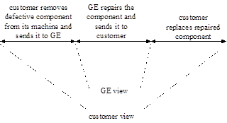
We must understand the customer’s perspective and expectations regardless of how much of it we control.

DFCI

Design For Customer Impact
Delivery span: the customers feel the variance, not the mean.

Six Sigma at the customer

Projects done by GE BB/GBs or customer BB/GBs, trained and/or mentored by GE BB/GBs
Address customer Ys
Address customer or GE Xs

	customer	GE
Ys	@ the customer	GE's DMAIC/DFSS projects
Xs	@ the customer	@ the customer

Lean Six Sigma

Hunt for waste

Define

Objectives:

• define the product or process to be improved
• identify customers and translate the customer needs into CTQs
• obtain formal project approval
• tools

• VOC tools and data techniques
• team charter
• high-level Process Map

Project selection
A good project should

• be clearly bound with defined goals
• be aligned with the business goals and initiatives
• be felt by the customer
• work with other projects for combined effects (may be driven by the funnel project of a BB)
• show improvement that is locally actionable
• relay to daily job

Sources of project ideas

• Quality Function Deployment (QFD)
• Customer Dashboards
• Surveys and Scorecards
• Active Beta Themes
• Other Projects Available for Leverage
• Brainstorming
• Analysis of Critical Processes
• Six Sigma Quality Project Tracking Database
• Discussions with Customer
• Financial Analysis
• Internal Problems

Step A: ldentify project CTQs

COPIS: customer centric view of the process

Customer: Whomever receives the output of your process (maybe internal or external)
Output: The material or data that results from the operation of a process.
Process: The activities you must perform to satisfy your customer’s requirements.
Input: The material or data that a process does something to or with.
Supplier: Whomever provides the input to your process.

Voice of the Customer (VOC)

VOC: what is critical to the quality of the process according to the customer.

	pros	cons
Surveys	Lower Cost approach Phone response rate 70 - 90% Mail surveys require least amount of trained resources for execution Can produce faster results	Mail surveys - can get incomplete results, skipped questions, unclear understanding Mail surveys - 20-30% response rate Phone surveys - interviewer has influential role, can lead interviewee producing undesirable results
Focus Groups	Group interaction generates information More in-depth responses Excellent for getting CTQ definitions Can cover more complex questions or qualitative data	Learning's only apply to those asked - difficult to generalize Data collected typically qualitative vs. quantitative Can generate too much anecdotal information
Interviews	Can tackle complex questions and a wide range of information Allows use of visual aids Good choice when people won’t respond willingly and/or accurately by phone/mail	Long Cycle Time to complete Requires trained, experienced interviewers

 

Customer Information Issues

• Real Needs vs. Stated Needs: Xerox: Focus on copiers or documents?
• Perceived Needs: A Hershey bar or Godiva chocolates?
• Intended vs. Actual Usage: Is a screwdriver also a hammer?
• Internal Customers: Turf wars and “not invented here.”
• Effectiveness vs. Efficiency Needs: “You want it right or you want it fast?”

The Affinity Diagram and Structure Tree can help to organize and translate VOC into customer needs.

Determine Priority CTQs

The specific needs statement provides the foundation for the 4 elements of the CTQ (Output Characteristic, Measure, Target/Nominal Value, Specification Limits).

Once CTQs are identified, the team should re-evaluate their charter. Will addressing the CTQs impact the issue(s) identified in the Problem Statement? Does the Scope of the Project allow for focus on the top 1 or 2 CTQs?

A successful project is related to one or more of the four vital customer CTQs:

• Customer Responsiveness/Communication
• Market Place Competitiveness — Product/Price/Value
• On-Time, Accurate, and Complete Customer Deliverables
• Product/Service Technical Performance

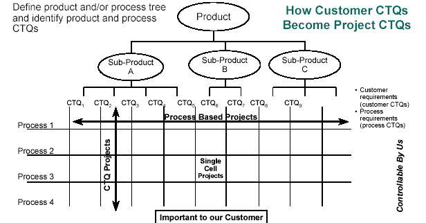
Product/Process Drill-Down Tree

The Process/Product Drill-Down Tree is a way to integrate CTQs with business strategy.

Step B: Charter

Objectives

• Clarifies what is expected of the team
• Keeps the team focused
• Keeps the team aligned with organizational priorities
• Transfers the project from the champion to the improvement team

Five elements of a charter

Business Case

Explanation of why to do the project

• Why is the project worth doing?
• Why is it important to do it now?
• What are the consequences of NOT doing the project?
• What activities have higher or equal priority?
• How does it fit with business initiatives and target?

Problem and Goal Statement

Description of the problem / opportunity or objective in clear, concise, measurable terms

• Problem Statement Purpose: Describes what is wrong
• What is wrong or not meeting our customer’s needs?
• When and where do the problems occur?
• How big is the problem?
• What is the impact of the problem?

Key Considerations/Potential Pitfalls

• Is the problem based on observation (fact) or assumption (guess)?
• Does the problem statement prejudge a root cause?
• Can data be collected by the team to verify and analyze the problem?
• Is the problem statement too narrowly or broadly defined?
• Is a solution included or implied in the statement?
• Would customers be happy if they knew we were working on this?
• Goal Statement Purpose: Defines the team’s improvement objective
• Defines the improvement the team is seeking to accomplish.
• Starts with a verb (reduce, eliminate, control, increase).
• Tends to start broadly — eventually should include measurable target and completion date.
• Does not assign blame, presume cause, or prescribe solution!

SMART

• Specific
• Measurable
• Attainable
• Relevant
• Time Bound

Project Scope

Process dimensions, available resources

• What process will the team focus on?
• What are the boundaries of the process we are to improve?
• What resources are available to the team?
• What (if anything) is out-of-bounds for the team?
• What (if any) constraints must the team work under?
• What is the time commitment expected of team members?

Milestones

Key steps and dates to achieve goal
A preliminary, high-level project plan with dates should be:

• Tied to phases of DMAIC process
• Aggressive
• Realistic

Roles

People, expectations, responsibilities

• How do you want the champion to work with the team?
• Is the team’s role to implement or recommend?
• When must the team go to the champion for approval? What authority does the team have to act independently?
• What and how do you want to inform the champion about the team’s progress?
• What is the role of the team leader (Black/Green Belt) and the team coach (Master Black Belt)?
• Are the right members on the team? Functionally? Hierarchically?

Step C: Process Map

Use COPIS: start with the customer and work backwards.
This is a high level process map:

• Name the process.
• Identify the outputs, customers, suppliers, & inputs.
• Identify customer requirements for primary outputs.
• Identify process steps.

Some CAP tools can also be used.

Measure

Objectives:

• select the measurable CTQs to improve
• map the process
• determine the specification limits for Y
• define the measure system and ensure the that it is adequate to measure Y through the use of a Gage R&R
• collect the data

Step 1: Select CTQ characteristics

Tools

The following tools are usable to select the CTQs on which to focus:

• QFD
• Fishbone
• Process Map
• Pareto Chart
• FMEA

A deplacer
Precision is the consistency of a process as measured by the standard deviation.
Accuracy is the ability to be on target as measured by the mean.
Process characterization describes the distribution of the data.

QFD (Quality Function Deployment)

QFDF is a structured methodology to identify and translate customer needs and wants into technical requirements and measurable features and characteristics.
It is used to identify CTQs.

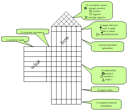
House of Quality

• step 1: find what the user wants (use the VOC tools described before) and write this list in the left hand column (the "what's")
• step 2: rate customer importance of each needs/wants (use factors in [1-5] or [1-10] range)
• step 3: list parameters that have an effect on the process/product (the "how's to satisfy" the "what's")
• step 4: evaluate the relationship between a factor and a customer need:

• double circle = strong = 9
• circle = medium = 3
• triangle = weak = 1

• step 5: define the target direction:

• upward arrow = more is better
• downward arrow = less is better
• circle = a specified amount

• step 6: indicate the target values, quantities and units, of the factors (they should come from the customer requirements)
• step 7: for each column, sum up the products ( customer importance * relationship ), this gives the technical importance of each parameter
• step 8: fill the correlation matrix between the parameters

• double circle = strongly positive
• circle = positive
• cross = negative
• double cross = strongly negative

Analyze the house of quality:

• blank row: we don't know how to satisfy a customer need
• blank column: the parameter has no impact on the customer needs
• no design constraint in how's
• resolve negative correlations
• finalize target values
• what parameters should be deployed to the next level of flowdown

QFD flowdown

Product:

• customer requirements → key functional requirements
• functional requirements → key part characteristics
• part characteristics → key manufacturing processes
• manufacturing processes → key process variables

Service:

• customer CTQs → key project deliverables
• key project deliverables → key process steps
• key process steps → key tasks

Use of QFD

Pitfalls:

• Do not use QFD for every project.
• Set the right granularity.
• Inadequate priorities.
• Lack of teamwork.
• Too much chart focus: the chart is the mean, not the objective
• "Hurry up and get done".

QFD must be regularly reviewed and updated.

FMEA

Preparation
1. Select Process Team
2. Develop Process Map and Identify Process Steps
3. List Key Process Outputs to Satisfy Internal and External Customer Requirements
4. List Key Process Inputs for Each Process Step
5. Define Matrix Relating Product Outputs to Process Variables
6. Rank Inputs According to Importance
FMEA Process
7. List Ways Process Inputs Can Vary (Causes) and Identify Associated Failure Modes and Effects
8. List Other Causes (Sources of Variability) and Associated FM&Es
9. Assign Severity, Occurrence and Detection Rating to each Cause
10. Calculate Risk Priority Number (RPN) for each Potential Failure Mode Scenario
Improvements
11. Determine Recommended Actions to Reduce RPNs
12. Establish Timeframes for Corrective Actions
13. Create “Waterfall” Graph to Forecast Risk Reductions
14. Take Appropriate Actions
15. Re-calculate All RPNs
16. Put Controls into Place

Risk Ratings: Scale: 1 (Best) to 10 (Worst)

• Severity (SEV)
  How significant is the impact of the Effect to the customer (internal or external)?
• Occurrence (OCC)
  How likely is the Cause of the Failure Mode to occur?
• Detection (DET)
  How likely will the current system detect the Cause or Failure Mode if it occurs?

Risk Priority Number:

• A numerical calculation of the relative risk of a particular Failure Mode.
• RPN = SEV x OCC x DET.
• This number is used to place priority on which items need additional quality planning.

The FMEA table contains the following columns:

• Process Step / Part Number
• Potential Failure Mode: Lists Failure Modes for each Process Step
• Potential Failure Effect: Lists the Effects of each Failure Mode
• SEV: Rates the Severity of the Effect to the Customer on a 1 to 10 Scale
• Potential Cause: Lists the Causes for each Failure Mode: Each Cause is Associated with a Process Input Out of Spec
• OCC: Rates How Often a Particular Cause or Failure Mode Occurs: 1 = Not Often, 10 = Very Often
• Current Controls: Documents How the Cause is Currently Being Controlled in the Process
• DET: Rates How Well the Cause or the Failure Mode can be Detected: 1 = Detect Every Time, 10 = Cannot Detect
• RPN: Risk Priority Number (RPN) is: Sev*Occ*Det
• Actions Recommended: Documents Actions Recommended Based on RPN Pareto
• Resp.: Designates Who is Responsible for Action and Projected Completion Data

Process Map

Process map: a graphical representation of steps, events, operations and relationships of resources within a process.

Use COPIS: start with the customer and work backwards.

Elements of a process

• Control: The material or data that is used to tell a process what it can or should do next.
• Mechanism: The resources (people, machines, etc.) that come to bear on a process to change the input to an output.
• Process Boundary: The limits of the process, usually identified by the inputs, outputs and external controls that separate what is within the process from its environment.

Benefits of Process Mapping

• Can reveal unnecessary, complex, and redundant steps in a process. This makes it possible to simplify and troubleshoot.
• Can compare actual processes against the ideal. You can see what went wrong and where.
• Can identify steps where additional data can be collected.

Most of the time, there are three maps:

• what we think may be happening
• what is actually happening
• what we want to be happening

ISO 9000 symbols

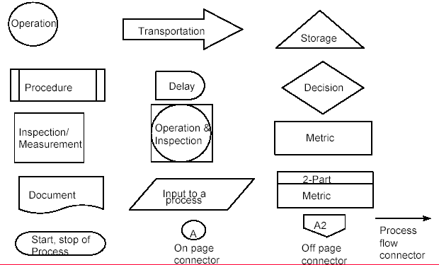
• prepare:
• Establish the process boundaries
• Observe the process in operation
• List the outputs, customers, and their key requirements
• List the inputs, suppliers, and your key requirements
• building the map
• determine the scope: what level of detail we want?
• determine the steps in the process: no order, no priority
• arrange the steps in order
• assign a symbol
• test the flow
• are the process steps identified correctly?
• is every feedback loop closed?
• does every arrow have a beginning and ending point?
• is there more than one arrow from an activity box? Perhaps it should be a diamond
• are all the steps covered?
• validate the map
• walk the process again
• ask the questions: What happens if…? What could go wrong? Who…? How…? When…?
• update map
• evaluating a Process Map
• does each step add value?
• are controls and measurement criteria in place?
• are “Re’s” occurring? Rework Revise Repeat Review
• is the step necessary?

Failure Modes and Effects Analysis: severity, occurrence, detection

See here.

Types of Data

• continuous: measured on a continuum or scale
• discrete         
• count: counted discreetly
• ordered categories: rankings or ratings
• binary: classified in one of two categories

Prefer continuous to discrete: continuous data often requires a smaller sample size than discrete data. For example, for delivery time, it is better to consider the actual times deviated from target rather than the number of late deliveries. Count and, maybe less easily, ordered categories, can be transformed in continuous data.

 

Step 2: Define performances standards

A Performance Standard is the requirement(s) or specification(s) imposed by the customer on a specific CTQ.
The goal of a performance standard is to translate the customer need into a measurable characteristic.

• Product/Process Characteristic
• Operational Definition
• Target
• Specification Limits
• Defect Definition

Operational Definition (SOP, Standard Operating Procedure): clear definition of what to measure (i.e. CTQ) and how to measure it.
Its purpose is:

• Remove ambiguity so that everyone has the same understanding
• Provides a clear way to measure the characteristic
• Identifies what to measure
• Identifies how to measure it
• Makes sure that no matter who does the measuring, the results are essentially the same
• Must be useful to both the company and the customer

Defect: the definition of a defect must be provided.
Try to get a continuous measurement instead of a discrete one.

Step 3: Measurement systems analysis

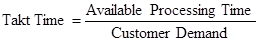
Takt time

Takt Time: The frequency at which each unit should be completed in order to meet customer demand. Takt Time establishes the necessary rhythm of the process.

Cycle time (touch time) = manual working time for one cycle of the process

Measure the cycle time for each step of the production flow.
If the cycle time is greater that the takt time, we cannot meet customer demand. If the cycle time is smaller than the takt time, the difference is the waiting time, this is an opportunity for improvement by redistributing the waiting time on other production steps.

Observation Sheet

The observation sheet is used to compute cycle time.
The observation sheet records:

• Set-up Time: Measure the set-up time and divide by the number of parts made between setups to get the set-up time per part.
• Manual Task Time: Measure and enter the hands-on time (human work) it takes for the operator to perform the operation with the machine (the process). Walking time is not included here.
• Auto-Run Time: Measure and enter the time from when the machine is switched on and it processes the part until the time when the machine returns to its original home position.
• Travel Time: Measure and enter the time it takes the operator to move to the next station and pick-up or put-down parts or tools. Leave this space blank if there is no travel time.
• Waste/Non-Value Added Activities: Record any non-value added activity that you observe and any recommendations for improvement.

Gage

In fact, we submit the output of a first process (the manufacturing process) to a second process (the measurement process). To address actual process variability, the variation due to the measurement system must first be identified and separated from that of the manufacturing process.

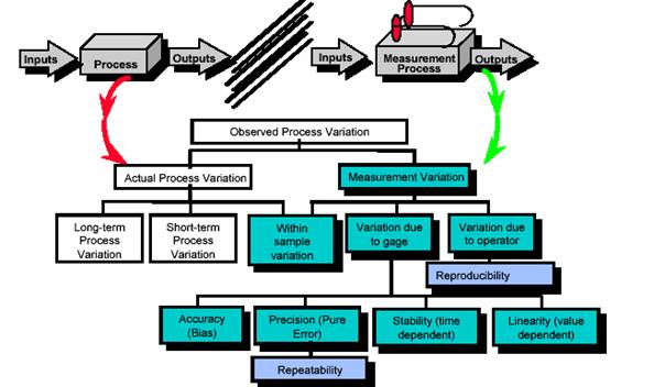
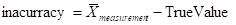
• accuracy: the differences between observed average measurement and a standard
• repeatability: variation when one person repeatedly measures the same unit with the same measuring equipment
• reproducibility: variation when two or more people measure the same unit with the same measuring equipment
• stability: variation obtained when the same person measures the same unit with the same equipment ever an extended period of time
• linearity: the consistency of the measurement across the entire range of the measurement system

 

The gage should have:

• precision: the gage should be able to resolve the tolerance into approximately ten levels ("the number of significant digits")
• accuracy: the gage noise must be less than the process noise ("the measured value is the real one")

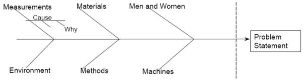
Elements of Measurement System Variability

• Men and Women
• Method
• Material
• Measurement
• Machine
• Environment

A Fishbone Diagram may be used to identify sources of variation in the measurement system.

Measurement Systems Analysis Checklist

1. What is the measurement procedure used?
2. Briefly describe the measurement procedure. What standards apply? Are used?
3. What is the "precision" (measurement error) of the system?
4. How has the precision been determined?
5. What does the gage (measurement system) Supplier state is the device’s:
= Discrimination (Resolution)?
= Accuracy (Bias)?
= Precision (Measurement Error)?
6. Do you have results of a:
= Test-Retest Study? (Determines Measurement Error or “lack-of-precision”)
= Gage R&R Study? (Allocates the error between device and operator(s))
If so, what are they? 7. Are different measurement systems (gages, scales, etc.) used to gather the
same data? Identify which data comes from which device.

Test-Retest Study

Best practice: do a test-retest study before the gage R&R study to get a quick look at the situation.
Repeatedly measure the same item with the same conditions, operator, device, and “location” on item and completely mount and dismount item for each measurement (“exercise” gage through full range of normal use.)
Perform 20 or more measures (10-15 may be OK if the measurements are expensive to perform).

• draw a plot chart
• device resolution:
  compute smeasurement it should be less than 1/10 of the tolerance
• device accuracy: if we know the true value of the test unit
  

Gage R&R

Collecting the Data
In order to get and estimate variation in the “Real” Measurement System:

• Follow actual process.
• Use the people that usually measure.
• Follow the planning for the job.
• Perform the study in the usual environment.
• Use the gages used for the job.

Gage Reproducibility (Appraiser Variation) & Repeatability (Equipment Variation)
s2equipment + s2appraiser = s2total(R&R)
Equipment Variation: (Sources of variation from within the process) the variation introduced into the measurement process from within one or more elements of the measurement process (within operator variation, within gage variation, within part variation, within method variation)
Appraiser Variation: (Source of variation from across the process) the variation introduced into the measurement process by effects going across the measurement process (different appraisers, different part configurations, different checking methods)

Rules of thumb

• %contribution (or Gage R&R StdDev) is ok below 2% and unacceptable above 8%
• %tolerance is ok below 10% and unacceptable above 30%
• number of distinct categories

signal-to-noise ratio = round(1.41*StdDevparts/StdDevGR&R)
1 no value for process control, part all look the same
2 can see two groups, high/low, good/bad
3 can see three groups, high/mid/low
4 acceptable measurement system

• effective resolution

control limits = +/- 3 <s>
more 50% of measurements are out of control limits

3 methods for Gage R & R computation

• short form
  a few operators measure the same parts

for each part, the range of the measure is computed. The sum of ranges is computed and divided by the number of parts to get the average range. Multiply by 5.15 and divide by the number of the following table to get the Gage R & R.

		Number of operators
		2	3	4
Number of parts	1	1.41	1.91	2.24
	2	1.28	1.81	2.15
	3	1.23	1.77	2.12
	4	1.21	1.75	2.11
	5	1.19	1.74	2.10
	6	1.18	1.73	2.09
	7	1.17	1.73	2.09
	8	1.17	1.72	2.08
	9	1.16	1.72	2.08
	10	1.16	1.72	2.08

the short form Gage R&R does not provide a way of separating gage repeatability and reproducibility.

• long form
• ANOVA
  to be written

Analyse

Objectives:

• Current process baseline has been calculated.
• The improvement goal of the project has been statistically defined.
• A list of statistically significant Xs has been generated as a result of analyzing historical data.

Step 4 - Establish process capability

Some distributions

• Uniform distribution
• Triangular distribution
• Normal distribution
• Exponential distribution

The distribution shape is not so important as to understand why the observed measure has this distribtuion and not another one.

Continuous data

Some definitions

• Probability:
  The sum of all probabilities is 1.

The symbols used for the population and for the sample are not the same:

	population	sample
mean (average)	(mu) =	(x bar) or(mu hat) =
standard deviation	(sigma)	or  (sigma hat)
variance	=	or  =

• Mode: most frequent value
• Range = Max - Min
• Mean :
• Deviation = (Xi - Xbar)
• Sum of square (SST) = sum of the square deviations
• Variance = average SST = s2 = S ( Xi - Xm )2 / N
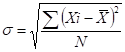
• Standard deviation = square root of the variance =
• Coefficient of variation = ratio of stdev to mean expressed as percentage =
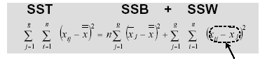
• Sum of square SST = SSw + SSb
  SST: sum of squares total
  SSW: sum of square within
  SSB: sum of square between
  

Tools

mettre chacun des tools dans un paragraphe indépendant

• Histogram to display variation in a process
  Purpose: To display variation in a process. Converts an unorganized set of data or group of measurements into a coherent picture.

When: To determine if process is on target meeting customer requirements. To determine if variation in process is normal or if something has caused it to vary in an unusual way.
How:

• Count the number of data points
• Determine the range (R) for entire set
• Divide range value into classes (K)
• Determine the class width (H) where H = R/K
• Determine the end points
• Construct a frequency table based on values computed in previous step
• Construct a Histogram based on frequency table
• Dot Plot to display variation in a process
  Purpose: To display variation in a process. Quick graphical comparison of two or more processes.

When: First stages of data analysis.
How:

• Create an X axis
• Scale the axis per the range in the data
• Place a dot for each value along the X axis
• Stack repeat dots
• Boxplot to get an overview of the data
  Purpose: To begin an understanding of the distribution of the data. To get a quick, graphical comparison of two or more processes

When: First stages of data analysis
How:

• minimum observation that fall within the lower Q1 - (Q3-Q1)*1.5
• Q1 - first quartile: 25% of observations is below
• median: 50% of observations is below
  if the number of observations is even, the median is the average of the two center values
• Q2 - third quartile: 75% of observations is below
• maximum observation that fall within the upper Q3 + (Q3-Q1)*1.5
• outliers: observations outside the lower and upper limits
• Run Chart to display data trends over time
  Purpose: To track process over time in order to display trends and focus attention on changes in the process

When:

• To establish a baseline of performance for improvement
• To uncover changes in your process
• To brainstorm possible causes for trends
• To compare the historical performance of a process with the improved process

How:

• Determine what you want to measure
• Determine period of time to measure and in what time increments
• Create a graph (vertical axis = occurrences, horizontal axis = time)
• Collect data and plot
• Connect data points with solid line
• Calculate average of measurements, draw solid horizontal line on run chart
• Analyze results
• Indicate with a dashed vertical line when a change was introduced to the process
• Multi-Vari Chart
  Purpose:
• To identify the most important types or families of variation
• To make an initial screen of process output for potential Xs
• Continuous Y, Discrete X

use it to see impacts of several families of variations: variation within (positional or location related), variation between (cyclical or batch/piece related) or variation time-to-time (temporal)

normality testing

• mean m = median = mode
• point of inflexion at s
• normal probability plot
• The result of the Anderson-Darling Normality Test tells if the data is normal or not. A p-Value of greater than 0.05 means the data is normal. A p-Value of less than 0.05 means that the data is not normal.

 

Most of the time when the data is not normal, this is because we are measuring the process as a whole and the results are the aggregation of several normal sub-results (i.e. the process is an aggregate of several sub-processes).

When the data is not normal, it is may be better to use the median and the span instead of the mean of the standard deviation to describe the data.
To describe the central tendency:

• mean
• median (if the distribution has a long tail or extreme outliers which inflate/deflate the average.)
• Q1 (if the data is skewed toward the low values) or Q3 (if the data is skewed toward the high values)

To describe the variation

• standard deviation
• span (P95 – P5) (used with long-tailed distributions)
• stability factor SF = Q1/Q3 (used with skewed distributions): the closer that the resulting number
• (Stability Factor) is to 1, the less variation is in the process; the closer the number is to 0 the greater the variation.

Normal distribution

computing in Excel
NORMSINV(1-DPO) compute Z from defect rate
1-NORMSDIST(Z) compute defect rate from Z

Z short term	Z long term	DPMO
2	0,5	308537,53
3	1,5	66807,23
4	2,5	6209,68
5	3,5	232,67
6	4,5	3,40

B2=A2-1,5
C2=(1-NORMSDIST(B2))*10^6

• Skewness
  Skewness is a measure of asymmetry. A value more than or less than zero indicates skewness in the data. But a zero value does not necessarily indicate symmetry.
• Kurtosis
  Kurtosis is one measure of how different a distribution is from the normal distribution. A negative value typically indicates a distribution more peaked than the normal. A positive value typically indicates a distribution flatter than the normal.

 

Zbench

Specs	LSL
	USL
Measurements	mean
	stdev
	Zusl	=(C2-C3)/C4
	Zlsl	=(C3-C1)/C4
	Pusl	=1-LOI.NORMALE.STANDARD(C6)
	Plsl	=1-LOI.NORMALE.STANDARD(C7)
	Ptotal	=SOMME(C8:C9)
	Zbench	=LOI.NORMALE.STANDARD.INVERSE(1-C10)

 

if data is normal, Minitab Six Sigma > process report
if data is not normal, minitab Six Sigma > product report

Discrete data

Definitions

• unit: number of elements inspected or tested (U)
• opportunity: an inspected or tested characteristic (OP)
• defect: a non-conformance (D)
• defect per unit: DPU=D/U
• total opportunities: TOP=U*OP
• defect per opportunity: DPO=D/TOP
• defect per million opportunities: DPMO=DPO*106
• Zlong term = 1 - NORMDIST(DPO)
• Zshort term = Zlong term + 1.5

Yield

Classical Yield (Yc): number of defect-free parts for the whole process divided by the total number of parts inspected. If we say the yield is 3/4 or 75%, we lose valuable data on the true performance of the process. This loss of insight becomes a barrier to process improvement.

First Time Yield (YFT): the number of defect-free parts divided by the total number of parts inspected for the first time. If we say the yield is 1/4 or 25%, we are really talking about the First Time Yield (FTY). This is a better yield estimate to drive improvement.

YTP is the percentage of units that pass through an operation without any defects. This is the best yield estimate to drive improvement.
Throughput Yield:
YTP = P(0) = e-DPU = e-2.25 = .1054 = 10.54%
percentage of units that pass through an operation without any defects. This is the best yield estimate to drive improvement.

YRT is the Rolled Throughput Yield
this is the yield of a process consisting of several steps
YRT is the product of the yield of each step

Quantification of Defects
inspection effectiveness

 

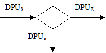
Percentage of likelihood of detecting a default: E
Submitted DPU Level: DPUS
Escaping DPU Level: DPUO
Observed DPU Level: DPUE
DPUS = DPUO + DPUE
DPUO = DPUS * E
DPUE = DPUS * (1-E)

Process capability

What is the best the process can be?

Special Versus Common Cause Variation

special (assignable) cause variation:

• It is non-random variation which can be assigned to specific causes
• It is controllable variation

 common (random) cause variation:

• It is an inherent, natural source of variation of the process
• It is not controllable variation

Rational Subgrouping

choose subgroups so that:

• There is maximum chance for the measurements in each subgroup to be alike. A subgroup should only contain common cause variation.
• There is maximum chance for subgroups to differ from one to the next. The difference between the subgroups is the special cause variation.

Z shift

The difference between a long-term data collection and short-term data collection can be demonstrated by Z shift. Over the short-term, common cause variation is present, but not special cause variation or mean shifts. The typical amount of variation added by including the long-term variation and mean shifts is 1.5σ.

Zshort term vs Zlong term

Use Anova 1-way in Minitab: SSW is the sum of squares for error, SSB is the sum of squares for group

Zlong term takes into account SST
Zshort term takes into account SSW

Long-term is what is actually going on in the process. It is defined by technology and process
control.
Short-term is the best the process can do. It is limited by technology only. This is the entitlement of the process.
Zshift = Zlt - Zst
The larger the Zshift , the greater the control problem. A typical value is 1.5.

Step 5 - Define performance objectives

Benchmarking is the process of continually searching for the best methods, practices and processes, and either adopting or adapting their good features and implementing them to become the "best of the best" possible benchmarking:

• Evaluating the Competition
• Determine the Best Process or Product
• Determining the Best Business Strategy
• Key Parameter within a Process
• Best Practices

Benchmarking should not be used as a single event, but should be utilized on a continuous basis.

benchmarking

• internal: similar activities within GE GE, but in different locations, departments, operating units, country...
• competitive: direct competitors selling to same customer base
• functional: organizations recognized as having world class processes regardless of industry

checklist

• identify process to benchmark

• Select process and define defect and opportunities.
• Measure current process capability and establish goal.
• Understand detailed process that needs improvement.

• select organization to benchmark

• Outline industries/functions which perform your process.
• Formulate list of world class performers.
• Contact the organization and network through to key contact.

• prepare for the visit

• Research the organization and ground yourself in their processes.
• Develop a detailed questionnaire to obtain desired information.
• Set-up logistics and send preliminary documents to organization.

• visit the organization

• Feel comfortable with and confident about your homework.
• Foster the right atmosphere to maximize results.
• Conclude in thanking organization and ensure follow-up if necessary.

• debrief & develop an action plan

• Review team observations and compile report of visit.
• Compile list of best practices and match to improvement needs.
• Structure action items, identify owners and move into Improve phase.

• retain and communicate

• Report out to business management and 6σ leaders.
• Post findings and/or visit report on local server/6σ bulletin board.
• Enter information on GE Intranet benchmarking project database.

Step 6 - Identify variation standard

Tools

• cause and effect (fishbone diagram)
• Pareto
• process mapping
• FMEA

Fishbone (cause and effect diagram)

Purpose:

• To provide a visual display of all possible causes of a specific problem

When:

• To expand your thinking to consider all possible causes
• To gain group’s input
• To determine if you have correctly identified the true problem

How:

• Draw a blank diagram on a flip chart.
• Define your problem statement.
• Label branches with categories appropriate to your problem.
  examples of categories:

• measurements, materials, men & women, mother nature (environment), methods, machines
• 4 Ps (...):Policies, Procedures, People, Plant

• Brainstorm possible causes and attach them to appropriate categories.
• For each cause ask, “Why does this happen?”
• Analyze results, any causes repeat?
• As a team, determine the three to five most likely causes.
• Determine which likely causes you will need to verify with data.

Pareto chart

Purpose:
To separate the vital few from the trivial many in a process. To compare how frequently different causes occur or how much each cause costs your organization.
When:
To sort data for determining where to focus improvement efforts.

• To choose which causes to eliminate first
• To display information objectively to others

How:

• Collect data (checksheets, surveys).
• Total results and arrange data in descending order.
• Draw and label a Pareto Chart.
• The X-axis shows the categories of problems.
• The left Y-axis shows the frequency/cost/impact in the units of measure (count, $, time, etc.).
• The right Y-axis shows the percentage (frequency of occurrence/total count of all occurrences).
• The bars show the value - frequency of occurrence.
• The line shows the cumulative percentage.
• Draw the largest frequency on the left and work your way down to the smallest on the right.
• Analyze results.
• Evaluate improvement effectiveness after change initiated by comparing before and after Pareto charts.

Process Map Analysis

• value-added work: steps that are essential because they physically change the product/service and the customer is willing to pay for them
• value-enabling work: steps that are not essential to the customer, but that allow the value-adding tasks to be done better/faster
• nonvalue-added work: steps that are considered non-essential to produce and deliver the product or service to meet the customer’s needs and requirements. Customer is not willing to pay for step.
• Internal Failure: Steps that are related to correcting in-process errors due to failures in current or prior step in the process. Example: Rework
• External Failure: Steps which relate to fixing errors in the product that the customer has found and has returned to you. Examples: Customer follow-up, Recall
• Control/Inspection: Steps for internal process review often referred to as “the checker-checking-the checker.” Examples: Inspection, Approval/review, Bureaucracy
• Delay: Steps where work is waiting to be processed at that step. Examples: Backlogs, Queues, Store, Bottlenecks
• Preparation/Set-Up: Steps that prepare work for a subsequent activity in the process. Examples: Entering into a computer, Retrieve policies/pricing
• Move: Steps that entail the physical transport or transmit of outputs between activities in a process. Example: Fax/mail

 

process time + delay time = cycle time

The delay may be due to:

• Gaps: responsibility for a given step in the process is unclear, or the process seems to go off track.
• Redundancies: duplication of efforts such as when two people or groups approve a document. Redundancies occur when different groups take action that they are unaware is being done somewhere else in the process.
• Implicit or unclear requirements: operational definitions do not exist or clear differences exist in perspective or interpretation.
• Tricky hand-offs: no check is in place to assure the process is continuing without delays. For example, Department A sends something to Department B but neither has a way to know if it was properly received.
• Conflicting objectives: the goals of one group cause problems or errors for another. For example, one group is focused on process speed while another is oriented to error reduction – the result may be that neither group accomplishes its objectives.
• Common problem areas: occurs when steps are repeated in a variety of places in process. Noting these areas may provide insight into potential solutions.

Draw a matrix:

• the columns are
• the workflow steps
• the total
• the total in percentage
• the rows are
• average time
• Value-Added
• Non-Value-Added subclassified into
• Internal Failure
• External Failure
• Control/Inspection
• Delay
• Prep/Set-Up
• Move
• Value-Enabling

FMEA

 

 

Hypothesis testing

An assertion or conjecture about one or more parameters of a population(s).
To determine whether it is true or false, we must examine the entire population. This is impossible!
Instead use a random sample to provide evidence that either supports or does not support the hypothesis
The conclusion is then based upon statistical significance
It is important to remember that this conclusion is an inference about the population determined from the sample data

Hypothesis Testing Protocol

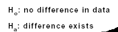
• state the null hypothesis H0 (using =, < or >)
• state the alternative hypothesis HA (using ≤, ≥ or ≠)
• test alternative hypothesis with Statistical Test
• based on the test result, we reject or fail to reject the null hypothesis Ho.

transfer following diagram

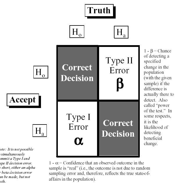
The P-Value:

• α is the maximum acceptable probability of being wrong if the alternative hypothesis is selected.
• The p-value is the probability that you will be wrong if you select the alternative hypothesis. This is a Type I error.
• Unless there is an exception based on engineering judgment, we will set an acceptance level of a Type I error at α = 0.05.
• Thus, any p-value greater than 0.05 means we accept the null hypothesis
  any p-value less than 0.05 means we reject the null hypothesis.

Seven examples of hypotheses

• the mean is on target
  Ho: μ = constant = T
  Ha: μ ≠ constant = T
• the variance is on target
  Ho: σ2 = constant
  Ha: σ2 ≠ constant
• two populations have the same mean
  Ho:µ1 = µ2
  Ha: µ1≠ µ2
• a population has a mean smaller than the mean of another population
  Ho: µ1 ≤ µ2
  Ha: µ1 > µ2
• two populations have the same variance
  Ho: σ12 = σ22
  Ha: σ12 ≠ σ22
• the populations have the same mean
  Ho: µ1 = µ2 = . . . = µn
  Ha: at least one not equal
• the populations have the same variance
  Ho: σ12 = σ22 = . . . = σn2
  Ha: at least one not equal

Hypothesis tests

			single X		several Xs
			continuous	discrete	continuous	discrete
single Y	continuous	normal	scatterplot single regression curve fitting (aka correlation)	T-test homogeneity of variance 1-way ANOVA	multiple regression	DOE 2, 3, 4, 5..-way ANOVA
		non-normal		homogeneity of variance Levine's Moods median correlation
	discrete		logistic regression	goodness of fit test of independence	multiple logistic regression	multiple logistic regression
several Ys			multivariate statistics

in the analysis phase, we only look at the xingle X / single Y, other tests will be seen in the improve phase
à mettre sous forme textuelle

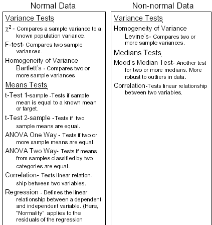
Hypothesis Testing: Continuous Y; Discrete X

to compare two or more distributions:

• Study stability

in Minitab , use Run Chart
look at graph shape
check p-values for clustering, mixtures, trends, and oscillations (Ho: Data is random, special causes not present; Ha: Data is not random, special causes present; so all p-values shall be greater than 0.05)

• Study shape

in Minitab, use Stat>Basic Statistics > Display Descriptive Statistics > Graphs... > Graphical summary in Minitab and look at shape and p-value for each distributions
p-value will indicate if data is normal or not: Ho: The data is normally distributed; Ha: The data is not normally distributed (p>0.05 indicate that the distribution is normal)

• Study spread
  in Minitab, stack the distributions in a column (and the distribution indices in another column), use Stat>ANOVA>Homogeneity of Variance
  to get the p-value:
• look at F-test (for 2 populations) or Bartlett's test (if more populations) is data is normal
• look at Levene's test if data is not normal

p-value < 0.05 means that the distributions are different

• Study Centering
  we compare the means of the populations
• to compare two populations
  the two populations must have the same variance
  in Minitab, Stat> Basic Statistics>2-Sample t
  (do not forget to check Assume Equal Variance)
  verify that the populations are different bu checking that
  - that 0 is not in the 95% confidential interval of mu Oper 1 - mu Oper 2 or
  - the p-value of the T-test (hypothesis is mu Oper 1 = mu Oper 2): p < 0.05
• to compare the mean of more than two populations
  the populations must have the same variance
  in Minitab, Stat> ANOVA>One Way
  check
  - that the 95% confidential intervals for the mean overlap
  - the p-value
  

look at excel document Analyze tool guide.xls

what about discrete data

non normal data:
look at plotchart
check that data is normal
sometimes, the data appears as not normal because the measurement resolution is not high enough
remove outlayers
try to find some possible subgroups
check that these groups are really different by performing a median test (Moods median test)
then performing HOV

data transformation should be used very carefully: it is easy to manipulate data which is meaningless.

pair testing :
we want to test if a change on a population of very different specimens has an impact
we must renormalize the data by computing the difference of the new and old values and perform

• a 1-sample T-test to see if 0 is in the 95% confidence interval of the mean or
• perform a T-test of the mean
  Stat > Basic Statistics > A Sample T and select Test Mean

how to draw the normality plot?

discrete Y - discrete X




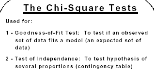
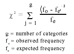
Chi-Square test
The population are different if p < 0.05. (If p>0.05 we reject the alternative hypothesis.)

in Minitab, to compute a sample size given the power of a test
Stat > Power and Sample Size > 1-sample t

 

comparison of means
1-sample T-test is used when comparing a population to a target
2-sample T-test is used when comparing two populations
ANOVA is used when comparing several populations

 

continuous Y - continuous X
use Scatter Plot to look at the data
in Minitab, Graph>Plot

in Minitab, Stat > Regression > Fitted Line Plot > Options > { Display Confidence Bands, Display prediction bands }
red lines indicate that we are 95% sure that the regression line is between these two lines
blue lines indicate that we are 95% sure that the measurement are between these two lines
n A confidence band (or interval) is a
measure of the certainty of the shape of
the fitted regression line. In general, a
95% confidence band implies a 95%
chance that the true line lies within the
band. [Red lines]
n A prediction band (or interval) is a
measure of the certainty of the scatter of
individual points about the
regression line. In general 95% of
the individual points (of the population on
which the regression line is based) will be
contained in the band. [Blue lines]

general linear model
see if the data is unbalanced
Stat > Tables > Cross Tabulation
if the data is unbalanced, we will us GLM
Stat > ANOVA > General Lineal Modal
the sum of squares depend on the order of the factors, the adjusted sum of square should be used instead.
p<0.05 indicates that the factor has an impact on the output
if the sum of squares is too small compared to the total sum of squares, this means that some factors have been forgotten

analysis of residuals
Stat > Regression > Residual plots...
What is the Normal Plot of Residuals drawing?

 

Improve

• To develop a proposed solution:
• Identify an improvement strategy
• Experiment to determine a solution
• Quantify financial opportunities
• To confirm that the proposed solution will meet or exceed the quality improvement goals:
• A pilot: includes one or more small-scale tests of the solution in a real-world business environment
• To statistically confirm that an improvement exists (hypothesis tests)
• To identify resources required for a successful full-scale implementation of the solution.
• To plan and execute full scale implementation including training, support, technology rollout, process and documentation changes.

Steps 7 - Screen potential causes

Steps 8 - Determine relationship

Improvement stategy

• operating parameters:
• Xs that can be set at multiple levels to study how they affect the process Y
• Changes in their settings impact the Y directly and influence variation
• May be continuous and/or discrete

use Statistical Breakthrough Strategy
you need to know how they are related to each other and to the Y to develop an
appropriate solution)

• develop a mathematical model, or
• determine the best configuration or combination of Xs
• critical elements:
• Xs that are independent alternatives
• Xs that are not necessarily measurable on a specific scale, but have an affect on the process

use Lean Process Improvement
you need to develop and test several practical alternatives to determine which is the best solution

• optimize process flow issues, or
• standardize the process, or
• develop a practical solution

Tools

depend on the problem sophistication (complexity, business impact, risk, data availability)

• basic
• fishbone
• boxplot
• linear regression
• hypothesis testing (z-test, t-test, ANOVA, chi-square, HOV)
• process map
• time order plots
• mistake proofing
• multi-vari plot
• force fields
• action work-out
• intermediate
• DOE (full, fractional)
• multi-variate regression
• advanced
• response surface
• Taguchi (inner/outer array)

Process of experimentation

There are seven steps:

• Define Project
• Identify responses
• Establish Current Situation
• Perform Analysis
• Identify factors
• Choose factor levels
• Select design
• Randomize runs
• Collect data
• Analyze data
• Draw conclusions
• Verify results
• Determine Solutions
• Record Results
• Standardization
• Determine Future Plans

DOE: Design Of Experiment

Possible ad-hoc improvement strategies:

• Stick-With-a-Winner

make a change: if this change results into an improvement, keep it; otherwise, change back and try another factor
→ major drawback : no guarantee to find the optimal solution, solution depends to some degree on which factor we decide to change first

• One-Factor-at-a-Time

Change only one factor at a time; once all the factors have been tested, include that resulted into an improvement in the final design
→ major drawback : multiple factor interactions are not taken into account

Replication: multiple observations performed with the different experimental units with the same factor settings

• to measure experimental variability, so we can decide whether the difference between responses is due to the change in factor levels (an induced special cause) or to common cause variability; to see more clearly whether or not a factor is important
• to obtain two responses for each set of experimental conditions → location, spread
• replication provides the opportunity for factors that are unknown or uncontrollable to balance out
• along with randomization, replication acts as a bias decreasing effect

Repetition: multiple observations performed with the same experimental unit
Randomization: assign the order in which the experimental trials will be run using a random mechanism

• averages the effect of any lurking variables over all of the factors in the experiment
• helps validate statistical conclusions made from the experiment

Analyzing a full factorial - replicated design

plot the raw data

• display run chart to see possible lurking variable
• display graphic statistic of the measures
  check if data is normal
• draw boxplot for the consolidated factor settings
• draw boxplots for each parameter to see which parameters have the highest impact
• compute the pooled standard deviation (square root of the average of the variances for each factor setting)
  this is why we need replicated measures
• use ANOVA one-way (for the consolidated factor settings) to see what is the variation due to parameter change and the variation due to process/measurement
  (to not forget to store the residuals, they will be used later)
  we must verify that the parameters have an impact (p<0.05, null hypothesis is that the populations of each experiment are the same)
  compute the residuals

plot the residuals

• display run chart of the residuals
• plot the residuals against the average
• plot the residuals on a normal probability scale
  check that they are normal

examine factor effects

• main effect plots

factor effect = average for the high setting - average for the low setting
a Factor Effect is the change in response due to a “two-unit” (-1 to +1) change in the factor.
a Factor Coefficient is the change in response due to a “one-unit” (-1 to 0 or 0 to +1) change in the factor.
Factor Coefficient = Factor Effect / 2

• interaction plots
• perform Stat > DOE > Factorial Plots to display
  (if the buttons are grayed out, use Stat > DOE > Create Factorial Design to create a DOE and ignore it)
• the main effects
• the interactions
• (the cube have no real interest)

confirm impressions with statistical procedures

• perform Stat > DOE > Analyze Factorial Design
  the significant parameters have a p-value less than 0.05
  coded units: parameters are normalized in the [-1,1] range
• it is also possible to use Stat > ANOVA > General Linear Model
  this shows the importance of each parameters, but not the interactions, they are in the error sum of square
  to see the interactions, add the factors A*B, A*C, B*C and A*B*C (it is not necessary to create the corresponding columns, Minitab will handle these products automatically)
  the factors having an impact are the ones with p < 0.05 and the sum of squares are the most significant (both criteria should be consistent, small p-value should be high sum of squares)

summarize conclusions

• List all the conclusions you have made during the analysis.
• Interpret the meaning of these results. For example, relate them to known physical properties, engineering theories, or your own personal knowledge.
• Make recommendations.
• Formulate and write conclusions in simple language.

 

at the bottom of the Run Chart; there are four p-values, they should all be less than 0.05.

Compute Prediction Model

keep only the significant factors
step 1: prepare a reduced design matrix
step 2: define custom design
step 3: run Factorial Analysis using Standard Deviation as response
step 4: build prediction model using significant factors
step 5: explore prediction models
optimize center (mean) and spread (standard deviation)
step 6: determine factor settings

Reducing size of experiments

 

• half factorial design: the last factor is the product of the other ones

e.g. for four parameters, D is equal to ABC, but it will be impossible to separate the effects of D and ABC, the effect of A and BCD, AB and CD, ABCD and the mean..., but effects of the combination of more than 2 factors to not exist in reality

• screening design
  we choose the next power of 2 and perform a full factorial for the first factors, the last ones are computes as product of the first ones
• Placket-Burman design

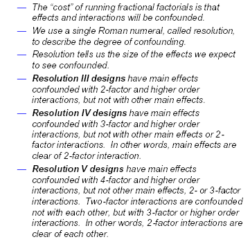
resolution
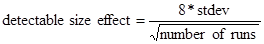
Detectable Effect Size: smallest effect we can consistently detect with the current number of experimental runs
First we must identify the current level of variability (standard deviation) for each response variable.

 

Step 9 - Establish operating tolerance

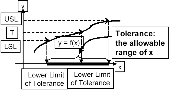
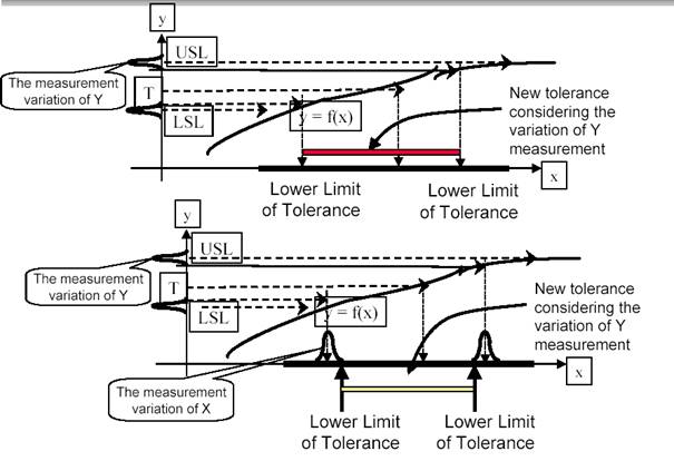
Tolerancing

Step 8 provided the experimental techniques to establish the relationship between the measurable Y characteristics and the controlling X factors.
Step 9, those relationships, so-called transfer functions, will be used to define the key operating parameters and tolerance to achieve the desired performance of the CTQs.

simulation

Simulation

• advantages

no need to build a prototype, make an experiment
does not disturb the system
no destruction in case of destructive test

• disadvantages

requires a good model

methodology for modeling and simulation process

• Specify - understand the problem to be studied and objective of doing simulation. Develop a project plan and get customer sign-off.
• Develop - describe model based on expert interviews and observation of process.
• Quantify - collect data needed to define process properties.
• Implement - prepare software model.
• Verify - determine that computer model executes properly.
• Validate - compare model output with real process (if it exists).
• Plan - establish the experimental options to be simulated.
• Conduct - execute options and collect performance measures.
• Analyze - analyze simulation results.
• Recommend - make recommendations.

Crystal Ball
http://sixsigmacafe.research.ge.com

Control

Objectives

• to make sure that our process stays in control after the solution has been implemented.
• to quickly detect the out of control state and determine the associated special causes so that actions can be taken to correct the problem before non-conformances are produced.

process entitlement: the best that can be achieved with the current technology of our process

Process Control System:

• Defines the actions, resources, and responsibilities needed to make sure the problem remains corrected and the benefits from the solution continue to be realized.
• Provides the methods and tools needed to maintain the process improvement, independent of the current team.
• Ensures that the improvements made have been documented (often necessary to meet regulatory requirements).
• Facilitates the solution's full-scale implementation by promoting a common understanding of the process and planned improvements.

Key Steps in Developing a Process Control System

• Complete an implementation plan:

• Plan and implement the solution and develop a method to control each vital X or key sources of variation
• Define all possible areas that may require action in order to control the process X and then determine the appropriate course of action to take

• Develop a data collection plan to confirm that your solution meets your improvement goals:

• Establish ongoing measurements needed for the project Y and create a response plan to follow in case process performance falls below established standards

• Communicate your strategy:

• Document the process and control plan to ensure process standardization and the continuation of the solution's benefits

• Train personnel.
• Run the new process and collect the data to confirm your solution.

Step 10 - define and validate measurement system on Xs in Actual Application

define and validate the measurement system on Xs in the actual application.
deliverable: measurement system is adequate to measure Xs.

we use the same tool as the ones used in step 3 to measure the Y

Step 11 - determine process capability

determine process capability.
deliverable: determine post-improvement capability and performance (Zst and Zlt).

Calculate post-improvement capability of performance based on the technique described in Step 4.
Confirm improvement goal established in Step 5 has been realized on the Y.
If not, go back to Step 6 to look for additional sources of variation.

Step 12 - Implement process control

quality plan
key questions

• why monitor?
• what should I monitor?
• output measures
• process measures
• input measures
• how much data do I collect?
• how can I detect changes in process variation or capability?
• what do I do if I detect a change?
• if the process is in control and capable, are my customers still satisfied?

risk management

• Identify the risk elements & the risk types.
• Cost
• Technology
• Specification
• Marketing
• Installation
• Assign risk ratings to the risks:
• Rate probability of occurrence (1 to 5):
• Rate consequence of occurrence/impact (1 to 5):
• Risk factor score — consequence x probability = 1 to 25.
• Prioritize the risks:

• HIGH Risk = RED Risk = Score of 16 to 25
• MEDIUM Risk = YELLOW Risk = Score of 9 to 15
• LOW Risk = GREEN Risk = Score of 1 to 8

• Identify the risk abatement plans (high and medium risks).
• Incorporate the risk abatement plan into the work plans.
• Track the risk score reductions and abatement actions vs. plan.
• Continuously update for new risks and reduction of old risks.

mistake proofing (poka yoke)

• a technique for eliminating errors
• make it impossible to make mistakes

• defects is the result of an error
• error is the cause of defects

 

Principles for Mistake Proofing:

• Respect the intelligence of workers.
• Take over repetitive tasks or actions that depend on constantly being alert (vigilance) or memory.
• Free a worker’s time and mind to pursue more creative and value-adding activities.
• It is not acceptable to produce even a small number of defects or defective products.
• The objective is zero defects.

Ten Types of Human Error

• Forgetfulness (not concentrating).
• Errors in mis-communications (jump to conclusions).
• Errors in identification (view incorrectly...too far away).
• Errors made by untrained workers.
• Willful errors (ignore rules).
• Inadvertent errors (distraction, fatigue).
• Errors due to slowness (delay in judgment).
• Errors due to lack of standards (written & visual).
• Surprise errors (machine not capable, malfunctions).
• Intentional errors (sabotage — least common).

Human Error-Provoking Conditions

• Adjustments.
• Tooling/tooling change.
• Dimensionality/specification/critical condition.
• Many parts/mixed parts.
• Multiple steps.
• Infrequent production.
• Lack of, or ineffective standards.
• Symmetry.
• Asymmetry.
• Rapid repetition.
• High volume/extremely high volume.
• Environmental conditions:

• Material/process handling
• Housekeeping
• Foreign matter
• Poor lighting

Mistake Proofing Techniques

Technique	Prediction/Prevention	Detection
SHUTDOWN	When a mistake is about to be made	When a mistake or defect has been made
CONTROL	Errors are impossible	Defective items can not move on to the next step
WARNING	That something is about to go wrong	Immediately when something does go wrong

Mistake Proofing Steps

• Identify Problems

• Brainstorming.
• Customer returns.
• Defective parts analyses.
• Error reports.
• Failure Mode and Effects Analysis (FMEA).

• Prioritize Problems

• Frequency.
• Wasted materials.
• Rework time.
• Detection time.
• Detection cost.
• Overall cost.

• Seek out the Root Cause

• Do not use mistake proofing to cover-up problems or to treat symptoms.
• Use mistake proofing to correct errors at their source.
• Other methods to determine the root cause are:

• Ask “why” five times
• Cause and effect diagrams
• Brainstorming
• Stratification
• Scatterplot
• Create Solutions

• Make it impossible to do it wrong.
• Cost/benefit analysis:

• How long will it take for the solution to pay for itself?

• Thinking outside of the box.

• Measure the Results

• Have errors been eliminated?

• Why or why not?

• What is the financial impact?

control plan

A good Control Plan will incorporate at least:

• Customer-driven Critical-To-Quality (CTQs).
• Input & Output variables.
• Appropriate tolerances (specifications for CTQs).
• Designated control methods, tools and systems:

• SPC
• Checklists
• Mistake proofing systems
• Standard Operating Procedures
• Manufacturing/Quality/Engineering Standards

• Reaction plan.

control charts

Control charts:

• Are used to monitor both inputs to process, parameters of a process, or process outputs (Xs and Y)
• Are used to recognize when a process has gone out of control
• Are used for identifying the presence of special cause variation within a process
• Do not tell us if we meet specification limits
• Neither identify nor remove special causes

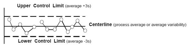
3σ-level control limits:

• Created by Shewhart to minimize two types of mistakes
• Placed empirically because they minimize the two types of mistakes

• Calling a special cause of variation a common cause of variation
  Missing an chance to identify a change in the process)
• Calling a common cause of variation a special cause of variation
  Interfering with a stable process, wasting resources looking for special causes of variation that do not exist

• Are not probability limits

Two Types of Control Chart

• variable chart (continuous)

Uses measured values
Generally one characteristic per chart.
More expensive, but more information.

• attribute chart (discrete)

Pass/Fail, Good/Bad, Go/No-Go information.
Can be many characteristics per chart.
Less expensive, but less information.

• process focused chart

Monitors several parts from same process
Measures deviation from nominal/target
Typically an I & MR chart monitoring several characteristic of several parts

Selecting the Appropriate Control Chart

• variable chart

• high volume
  X-bar and R charts
  X-bar: average of the sample
  R: range of the sample (max of sample – min of sample)
  if sample size is greater than 5, a S chart should be used in place of the R chart
• low volume
  individuals & moving range charts
  individual: the value of the sample
  moving range: the different between the value of the sample and the value of the previous sample

• attribute chart (defect = a single characteristic that does not meet requirements; defective = a unit that contains one or more defects)

• constant lot size

• defects
  C chart
• defectives
  NP chart

• variable lot size

• defects
  U chart
• defectives
  P chart

The Process is “Out-of-Control” if...

• Four Western Electric Rules

• A point is outside the control limits.
• 2 out of 3 consecutive points > 2 σ away from the mean on the same side.
• 4 out of 5 consecutive points > 1 σ away from the mean on the same side.
• 9 consecutive points are on one side of the mean.

• Minitab Rules

• one point more than 3 σ from the center line
• nine points in a row on the same side of center line
• six points in a row, all increasing or all decreasing
• fourteen points in a row, alternating up and down
• two out of three points more than 2 σ from center line (same side)
• four out of five points more than 1 σ from center line (same side)
• fifteen points in a row within 1 σ sigma of center line (either side)
• eight points in a row more than 1 σ from center line (either side)

process focused chart

• Define the process (general is better than specific).
• Identify the parameters that measure performance.
• Gather data in production sequence.
• Record variable data as a deviation from nominal/target.
• Analyze for patterns.